


brain of mat kelcey...
FiLM INR oscillator
July 18, 2026 at 07:00 PM | categories: eurorack, tiliqua, fpgaimplicit neural representations
parking cdcc
my long running tiliqua project has cached dilated causal convolutions (CDCC); a large dilated conv net that leans heavily on activation caching to get inference speeds of 192kHz
the initial goal for CDCC was to be an effect, like a delay or reverb, which requires the ability to integrate over a long sequence.
was tinkering with this architecture trying to get some psram stuff working when i suddenly realised something; the cdcc approach is great for long range integration but for a plain "stateless" oscillator you don't need any of that.
an oscillator is way more direct than an effect; it just needs to map from phase and some conditioning variables to a waveshape and that's a classic implicit neural representation (INR)
dataset
the test dataset is the same one i started with for CDCC.
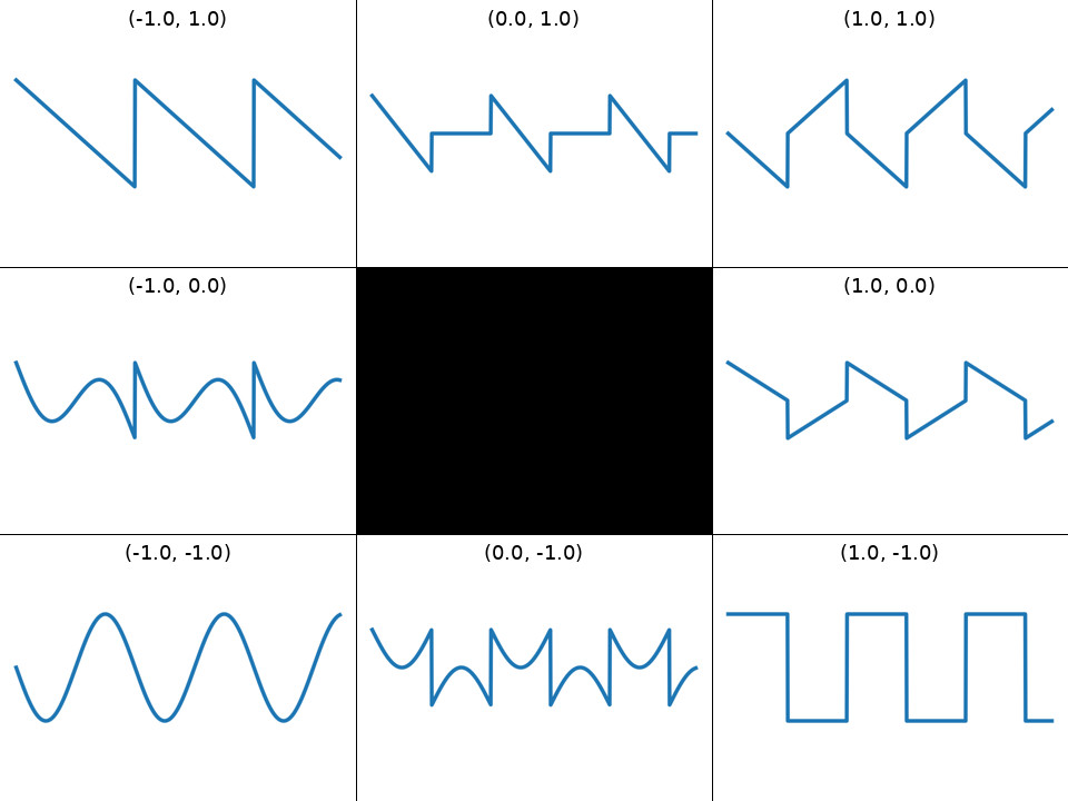
the output waveshape is represented by a 2d embedding. training examples are generated in numpy by sampling two endpoints, then picking a point in between, and generating a constant power cross fade interpolation. we intentionally use waves that have interesting interpolated points. we sample data over a range of octaves.
neural oscillator
my baseline for INR was just 3 inputs; the 1d phase value & the 2d embedding. and it didn't work at all... the network needs more to bite into than just a single phase value!
the next version was 4 inputs; a quadrature sin/cos for the phase & the 2d embedding. this did a lot better ( as i knew from the cdcc work ) and i thought, if sin/cos does well, why not other basis values too? and of course, this is already well studied under random fourier features (RFFs)
the idea is just to sample a random bank of basis frequencies and have the phase sweep through them, calculating the quadrature sin and cos pairs for each. the job of the network then is to represent a mixing of these basis values.
the initial model was...
- 3 values for the input; 1d input phase ( a sawtooth which acts as an index into the bank ) and 2d embeddings
- a mapping from the phase to 64 random fourier basis values; calculating the sin and cos of each to make a 128d feature vector.
- concatenation of the 128d RFF feature vector & the 2d embedding
- finishing with a small MLP
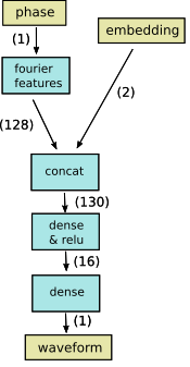
this gives a pretty good result but has some key problems we can fix...
feature imbalance and FiLM to the rescue
the main problem i found is that there is a bit of an imbalance between the inputs.
we have 128D representing the phase and only 2D for the embedding part. it's easy for the model to get a bit stuck just ignoring the embedding.
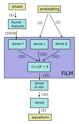
turns out there's a much better way to use the embeddings to condition the RFFs; rather than concat them, we can use the embeddings to modulate the fourier features.
specifically we learn three projections using dense layers, all to the same output dimension
- rff -> F
- embeddings -> gamma
- embeddings -> beta
and then combine them as output = (1+gamma) . F + beta
this now means the embeddings are being used to rescale and offset the RFFs
( notice that we parameterise as 1+gamma. this allows us to init weights for gamma and beta as 0 turning the entire linear function into a noop at the start of training )
i first saw this in FiLM: Visual Reasoning with a General Conditioning Layer ( Feature-wise Linear Modulation )
the qkeras models looks like ...
__________________________________________________________________________________________________
 Layer (type)                Output Shape                 Param #   Connected to
==================================================================================================
 input_1 (InputLayer)        [(None, None, 3)]            0         []

 phase (Lambda)              (None, None, 1)              0         ['input_1[0][0]']
 rff (QRandomFourierFeature  (None, None, 1024)           512       ['phase_q[0][0]']
 film0_F (QDense)            (None, None, 32)             32800     ['rff[0][0]']

 embed (Lambda)              (None, None, 2)              0         ['input_1[0][0]']
 film0_gamma (QDense)        (None, None, 32)             96        ['embed_q[0][0]']
 film0_beta (QDense)         (None, None, 32)             96        ['embed_q[0][0]']

 film0 (FiLM)                (None, None, 32)             0         ['mlp0[0][0]',
                                                                     'film0_gamma_q[0][0]',
                                                                     'film0_beta_q[0][0]']
 qrelu0 (QActivation)        (None, None, 32)             0         ['film0[0][0]']

 mlp1 (QDense)               (None, None, 32)             1056      ['qrelu0[0][0]']
 qrelu1 (QActivation)        (None, None, 32)             0         ['mlp1[0][0]']

 mlp2 (QDense)               (None, None, 32)             1056      ['qrelu1[0][0]']
 qrelu2 (QActivation)        (None, None, 32)             0         ['mlp2[0][0]']

 y_pred (QDense)             (None, None, 1)              33        ['qrelu2[0][0]']

==================================================================================================
Total params: 35651 (139.26 KB)
this gives a much better smoother result.
initially though i thought i wouldn't be able to use this approach since it adds more compute ( the gamma and beta dense layers ) but then i noticed a whooping optimisation!
lookup tables!
the biggest layer by far is the FiLM dense_F; it has to map from 1024 RFFs to a 32d output
but note that phase -> RFF -> FiLM dense_F is only dependant on phase. and since everything here is being quantised there's only a fixed number of values that phase can take. so we can just materialise the whole lot and treat it as a lookup. ( we have more than enough space for it in psram! )
AND note that the size of table depends on only two things
- the quantisation of the phase ( which dicates the number of entries ) and
- the size output dim of dense_F ( which dicates the size of each entry ).
which makes the number of RFFs only a concern at training since, for inference, it gets contracted away into lookup table. that's a HUGE win since it was the largest component of everything.
also note that this is something we couldn't do with the concatenation case ( though i guess we could have projected down between the RFFs & the concat and cached that instead... )
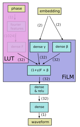
for v1 of this i built the table at module startup by sweeping sweep thru the phase values and populating the table in psram. this was fine until the table got big enough that the startup time was getting annoying.... at that point i switched to building it fully offline as a .bin file and adding it to the archive as something to directly load in psram.
activation fn?
did a fair bit of experimenting with what activation function to use for the MLP dense layers.
tried relu vs leakyrelu vs siren ( introduced in Implicit Neural Representations with Periodic Activation Functions )
for this problem at least siren only made a very minor improvement. have already seen it doing much better on ( work in progress ) more complex waveshaping so expect it to be important for the next piece of work.
training
for training i took the same approach as CDCC; it's worked for me a couple of times now..
- pretrain f32 keras model
- finetune fixed point qkeras model
- export weights for amaranth inference
felt like a lot more messing around this time getting bit exactness between qkeras and amaranth, especially with things like the LUTs
siren in particular required another LUT for the trig functions and had to roll my own STE (straight through estimation) stuff for it since qkeras didn't support it.
losses
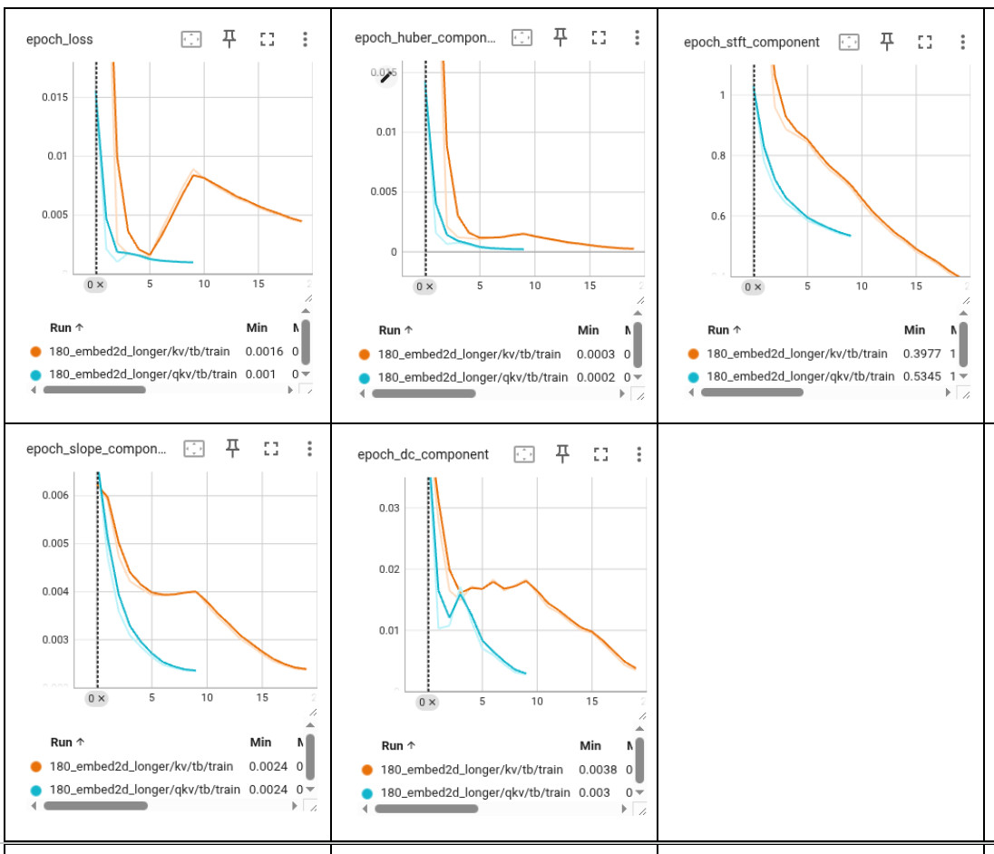
also spent a bunch of time tinkering with loss functions ( mainly since training for spectral correctness is new to me... )
main loss was a combination of huber & short time fourier transform (STFT) with stft needed a lot of tuning, and i still don't think it's quite right.
( and spectral stuff is so weird, it's bizarre to have cases of low spectral loss, and higher huber loss, and have the wave look worse but sound better (?!?!) )
the key i noticed was to let huber stabilise things then ramp up the STFT loss ( which switches the huber from being the waveshaping to be more about phase locking ). if i started training with stft immediately it was unstable.
also included some aux losses that, to be honest, probably didn't make much difference to things.
- a slope loss; simple first order loss ; instead of the absolute difference, try to matching the rate of change over two steps.
- dc offset loss; output should also be zero centered so added this.
not sure either did anything, was mainly curious.
device inference and util
most of amaranth code was taken from CDCC. did quite a bit of tuning around the lane-parallel and weight banks for the MAC stuff. all fits comfortably on the device.
DP16KD:32%  MULT18X18D:42%  ALU54B:0%  TRELLIS_FF:37%  TRELLIS_COMB:48%
Info: Router1 time: 0h 00m 36s
Info:  '$glbnet$audio_clk': 71.97 MHz (PASS at 50.00 MHz)
Info:        '$glbnet$clk': 89.00 MHz (PASS at 60.00 MHz)
demo
next steps
- v1 of CDCC was keras -> qkeras -> verilog
- v2 of CDCC was keras -> qkeras -> amaranth
- v1 of INR was keras -> qkeras -> amaranth
- maybe FiLM and an MLP even with siren isn't the right approach; maybe i should try RFF -> state space model (SSM) ?
- next version (SSM) will be jax -> amaranth ( since i have to patch qkeras a bit ( in terms of STE for LUT backprop ) have put more and more of
- RFF basis set is just randomly sampled. is there a way to analysis a bunch of the training data to get a better set of starting basis values? maybe a mix of random and some derived ones?
- get back to parametric capture stuff i was working before i got distracted with INR. it's currently tied up with the cdcc work but i think it's worth pulling out to a single project ( to support all these projects )
- am also keen to replicate some of the neural tangent kernel stuff given how well FiLM worked for me!